The Free On-line Stanford AI Class didn't have the programming problems that the in-person class did, due to lack of grading resources - but we did get a simple, optional, mini shredder challenge where it was suggested that we use NLP techniques to reassemble 19 vertical (2 character wide) slices of a paragraph back together in the right order. The popular approach was to simply produce some letter statistics (usually bigram) on english words, and then glue stripes together picking the addition that improves the score most.
Most of the approaches discussed afterwards on the aiclass Reddit involved getting a big chunk correct using machine techniques and then fixing up the last chunks by hand; my personal approach found "Claude" and "Shannon" recognizably, leaving very little hand-work. (Note that the actual shredder challenge was won by a team using a hybrid computer-vision/nlp/human approach, so one could argue that this is a state-of-the-art method.)
In my example, I grabbed /usr/share/dict/words and chewed it into statistics by hand; not very sentence like, but by pairing spaces with initial and terminal letters I got good word-assembly out of it. Later, I figured that a good example of "coding well with others" would be to actually use the widely acclaimed NLTK Natural Language Toolkit, especially if that showed that the additional effort of understanding an existing solution would have some measurable benefit towards executing that solution.
The first approach was to replace my dictionary extractor:
ascii_words = [word.lower().strip() for word in file("/usr/share/dict/words")
                    if word.strip() and not (set(word.strip()) - set(string.letters))]
with code that pulled the words from the Project Gutenberg sample:
import nltk
nltk.download("gutenberg")
ascii_words = nltk.corpus.gutenberg.words()
Then I reran the code (as a benchmark to see how much of a difference having "realistic" words-in-sentences probabilities would make.) Inconveniently (but educationally), it made so much of a difference that the first run produced a perfect reassembly of the 19 slices, with no need for further human work (either on the output data or on the code...) Still, there are a bunch of ad-hoc pieces of code that could be replaced by pre-existing functions - which should in theory be more robust, and perhaps also easier to share with others who are familiar with NLTK without forcing them to unravel the ad-hoc code directly.
A thread on nltk-users points out the master identifier index where one can find a bunch of tools that relate to word-pair bigrams, but also the basic nltk.util.bigrams that we're looking for. In fact, our existing code was a somewhat repetitive use of re.findall:
for ascii_word in ascii_words:
    for bi in re.findall("..", ascii_word):
        in_word_bigrams[bi] += 1
    for bi in re.findall("..", ascii_word[1:]):
        in_word_bigrams[bi] += 1
which turns into
for ascii_word in ascii_words:
    for bi in nltk.util.bigrams(ascii_word):
        in_word_bigrams["".join(bi)] += 1
(in_word_bigrams is a defaultdict(int); the join is necessary to keep this a piecewise-local change - otherwise I'd have to look at the later scoring code which uses substrings and change it to use tuples.)
The use of nltk.util.trigrams is nearly identical, replacing three more re.findall loops.
It turns out we can go another step (perhaps a questionable one) and replace the defaultdict above with nltk.collocations.FreqDist() giving this:
in_word_bigrams = nltk.collocations.FreqDist()
for ascii_word in ascii_words:
    for bi in nltk.util.bigrams(ascii_word):
        in_word_bigrams.inc("".join(bi))
In practice, most Python developers should be more familiar with defaultdict (those with long term experience might even have a bit of jealousy about it, as it wasn't introduced until Python 2.5.) One benefit of using FreqDist is that it includes a useful diagnostic method, .tabulate, which lets us confirm that the statistics are what we expect from english-language text:
print "In Word Bigrams:"
in_word_bigrams.tabulate(15)

In Word Bigrams:
  th   he   an   in   er   nd   re   ha   ou   at   en   hi   on   of   or
310732 284501 153567 147211 140285 134364 112683 103110 95761 88376 84756 82225 81422 77028 76968
and similarly for the other tables. Even better, adding one more line:
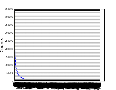
all_bigrams.plot()
uses matplotlib to show us a nice graph that again confirms our suspicion that bigram statistics have a tail, without having to get distracted by the mechanics of doing the plotting ourselves - some past nltk developer decided that frequency distributions were sometimes worth visualizing, and we get to take advantage of that.
Since the actual task involves coming up with the probability that a given partial combination of strips of text is in english, as the completely unscrambled one will be - bigram frequency counts aren't directly useful, we need to normalize them into probabilities. Again, this isn't much Python code:
bi_total_weight = sum(all_bigrams.values())
norm_bigrams = dict(((k, v/bi_total_weight) for k,v in all_bigrams.items()))
but the nltk.probability module has a class that performs this conversion directly:
norm_bigrams_prob = nltk.probability.DictionaryProbDist(all_bigrams, normalize=True)
A quick loop to print out the top ten from both shows that
DictionaryProbDist is implementingThere is an interface difference; instead of dictionary lookup, DictionaryProbDist provides .prob() and .logprob() methods. Nothing else that leaps to the eye as helpful to this particular problem - but it's useful to notice the .generate() method, which is proportional sampling with replacement - which is basically the core of the Particle Filter algorithm.
For the final step, we need to apply our bigram (and trigram) probabilities to our partially assembled bits of text, so that we can greedily pick the combinations that are approaching english the most quickly. However, we have bigrams that appear in the target that don't appear in the model corpus; as explained in Unit 5, Section 21, if you assign those missing values a probability of zero, they falsely dominate the entire result. (If you use the model that way anyhow, it does in fact come up with a poor combination of strips.)
In the original implementation, I assigned an arbitrary and non-rigorous "10% of a single sample" value, which was at least effective:
for i in range(len(word) - 1):
    # go back and do the smoothing right!
    s *= bigrams.get(word[i:i+2], 0.1/bi_total_weight)
return math.log(s)
It turns out that nltk.probability has some more useful surprises in store - we can simply use LaplaceProbDist directly, since k=1 is sufficient. It turns out that the general form is also called Lidstone smoothing so we could use LidstoneProbDist(gamma=k) if we needed to experiment further with smoothing; in the mean time,
norm_bigrams = nltk.probability.LaplaceProbDist(all_bigrams)
for i in range(len(word) - 1):
    s += bigrams.logprob(word[i:i+2])
return s
simply (and convincingly) "multiplies" probabilities (adding logs, just to get numbers that are easier to handle - that is, easier to read in debugging output.)
One interesting result of looking at the logs is that while the chosen strips are typically 2**15 to 2**90 more likely than the second best choice, once we've assembled "Claude Shannon founded" it jumps out that the best next choice (by a factor of "merely" 5) is actually to (incorrectly) add a strip on the left... so at least with the gutenberg corpus, the assemble-to-the-right bias actually helps reach the desired answer, so there's more room to improve the method. The numbers also tell us that it's a path problem, not a result problem - the evaluation function gives a 2**94 higher probability for the correct result than for the (still slightly-scrambled) result that the symmetric (but still greedy) version produces.
While it was certainly faster to code this up in raw Python the first time around - note that this was a single instance problem, with new but thoroughly explained material, where the code itself was not judged and would not be reused. Once you add any level of reuse - such as a second problem set on the same topic, other related NLP work, or even vaguely related probability work - or any level of additional complexity to the original problem, such as a result that couldn't be judged "by eye" - digging in to NLTK pays off rapidly, with dividends like
LaplaceProbDist)tabulate, plot)DictionaryProbDist.generate as relevant to Particle Filters.)LaplaceProbDist, util.bigrams)The last one is perhaps the most relevant benefit, because even though the code may perform identically, and the line counts are the same, the version that uses the NLTK-supplied abstractions should communicate more clearly to the next human reader of the code - an important "coding well with others" principle.